We are unable to give access to complete raw data-sets but have uploaded de-identifed snippets so that the key processes could be replicated.
Outlier detection
To ensure data quality while preserving natural variability, we implemented a conservative outlier detection approach based on robust scale estimation (Qn method). Rather than relying on the standard deviation method, which can be heavily influenced by extreme values themselves (Rousseeuw & Croux, 1993).
The Qn method works by calculating pairwise differences between observations and selecting a scaled quantile from these differences. This approach has been show to be a robust measure of dispersion that maintains resistance to contamination even when up to 50% of the data contains outliers, making it substantially more reliable than traditional methods in the presence of extreme values (Rousseeuw & Croux, 1993)
For each subject and variable combination, we established outlier boundaries by:
Lower bound = Median - (2.75 � Qn scale) Upper bound = Median + (2.75 � Qn scale)
The multiplier of 2.75 was deliberately chosen to implement a conservative threshold that retains most natural variability while excluding only the most extreme observations. All observations that were flagged as potential outliers were scrutinized by domain experts to confirm before removal.
Rousseeuw, P. J., & Croux, C. (1993). Alternatives to the Median Absolute Deviation.�Journal of the American Statistical Association,�88(424), 1273–1283. https://doi.org/10.1080/01621459.1993.10476408
Across all the variables analysed for future analysis, a range of 7 to 31 (0.91% to 4.13% of total observations for each test) observations were considered flags and subsequently removed prior to analysis.
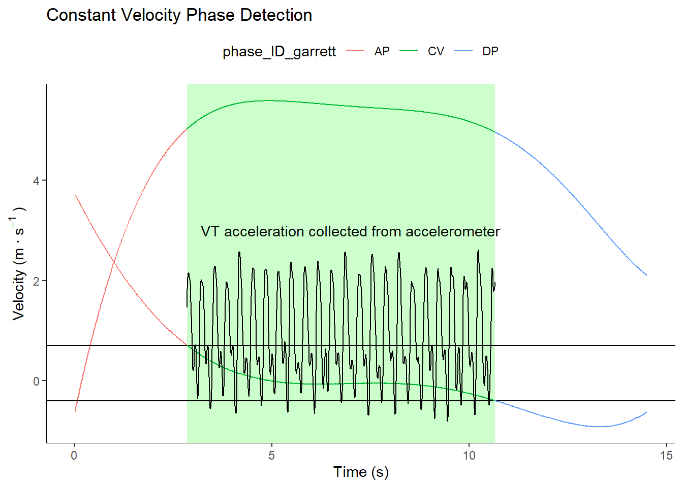
1) Constant Velocity identification
Below shows steps used to identify constant velocity during the High-intensity Intermittent-fixed Submaximal Run (HI-IR). Constant velocity was consistent with the method outlined by Garret et al.
Accelerometer data collected within the CV phase were then used to calculate player load calculations using formula outlined within the manuscript for all three vectors. Vertical accelerometer data was additionally used to calculate the number of steps that were achieved during the constant velocity phase, where the step detection method is outlined below.
2) Step detection and Normalization of High-intensity Intermittent-fixed Submaximal Run (HI-IR)
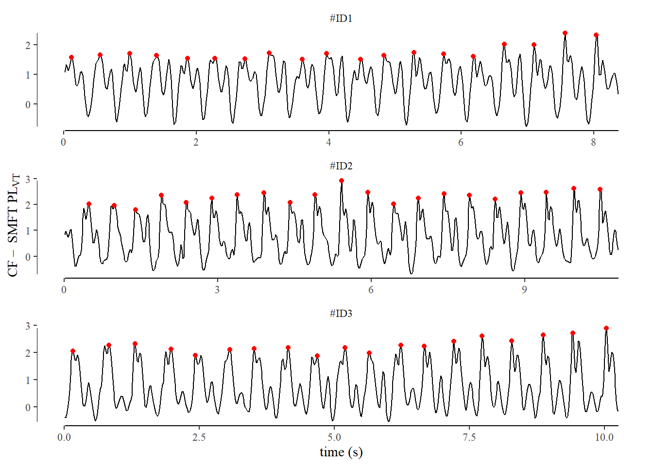
Prior to analysis, three trials were excluded from the study due to insufficient data. The exclusion criterion was set at a minimum of 6 steps identified during the constant velocity phase. This threshold was chosen to ensure at least three steps per leg were captured, which we deemed as bare minimum for accurate assessment of the collected parameters during constant velocity (44). Step identification was performed using vertical acceleration peaks from the 100Hz Inertial Measurement Unit (IMU) data. We employed components of a method described by Benson et al. (45), implemented using the pracma package. All identified peaks were visually inspected for each athlete-trial to ensure accuracy.
An example of this process is outlined below.
# load dataSD_url <-"https://raw.githubusercontent.com/R2mu/AdditionalMaterials/main/data_AddMat/exampleStepDetection.csv"stepDet<-fread(SD_url)# find peaks algorithm# settings chosen were based of visual inspection that most reliable identified peaks in contact across all individuals. find_peaks <-function(x,minPeakHeight=1.2) { peak_indices <- pracma::findpeaks(x, threshold =0, minpeakdistance =16,minpeakheight = minPeakHeight,zero ="+")[, 2] peak_indicator <-as.integer(seq_along(x) %in% peak_indices) return(peak_indicator)}# implementaion of find peaks across three sample players on a smoothed vertical acceleration signal can be seen below # Filtering was performed using a 4th order 25 hz low pass butterworth filterstepDet <- stepDet[,bw.25_acc.up:=round(filtfilt(butter(1,.25,type="low"), acc.up),2),by=.(ID) ][,peak:=find_peaks(bw.25_acc.up,minPeakHeight =1.2), by=.(ID)]
Visual representation of step detection. This was performed for each testing occasion to ensure appropriate detection across all players.
This was then summarised along with other key Player load derived measures to make sure a minimum of 6 steps was used for further analysis. Below is an example of how this was summarized for each player on each testing occasion.
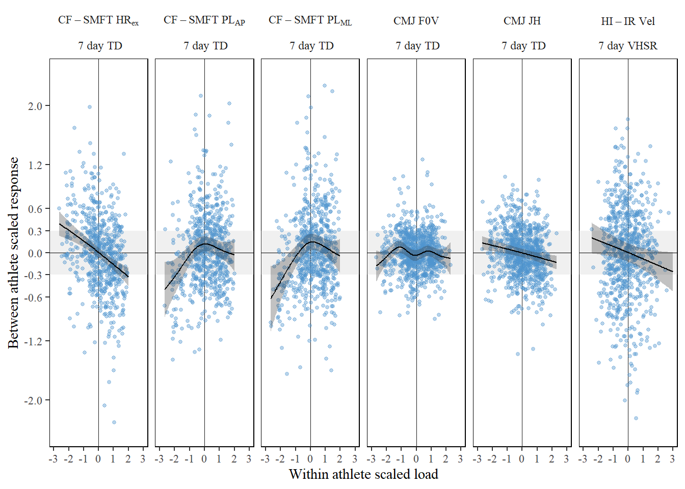
As both duration and velocity of the HI-IRplateau directly influence accumulated accelerometer-vector loads and were observed to vary from week-to-week, an adjusted estimate was developed. Below is an outline of the steps followed.
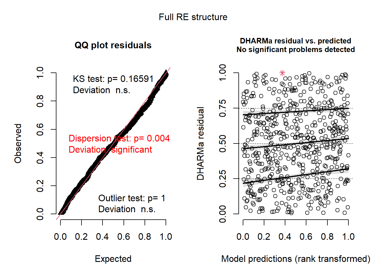
Significant improvements from the null model to the fully specified are noted above, we which were also assessed on the hold out data below.
model_list <-list(null_model = adj.VT_null,sparse_re = adj.VT_sml, # simplified random effects structurefull_re = adj.VT_fs # maximal random effects structure# acc_AP = log_adj_AP, place holder for acc.fwd# acc_ML = log_adj_ML place holder for acc.side)for (model_name innames(model_list)) { current_model <- model_list[[model_name]]tst_dat = test_data[,preds:=predict(current_model,.SD) ][!is.na(preds), ][,diff_sq := (logVT-preds)^2 ] rmse = tst_dat[,.(RMSE=sqrt(mean(diff_sq)))]print(paste0("test data RMSE for ",model_name,": ",round(rmse,2)))}
[1] "test data RMSE for null_model: 0.25"
[1] "test data RMSE for sparse_re: 0.13"
[1] "test data RMSE for full_re: 0.12"
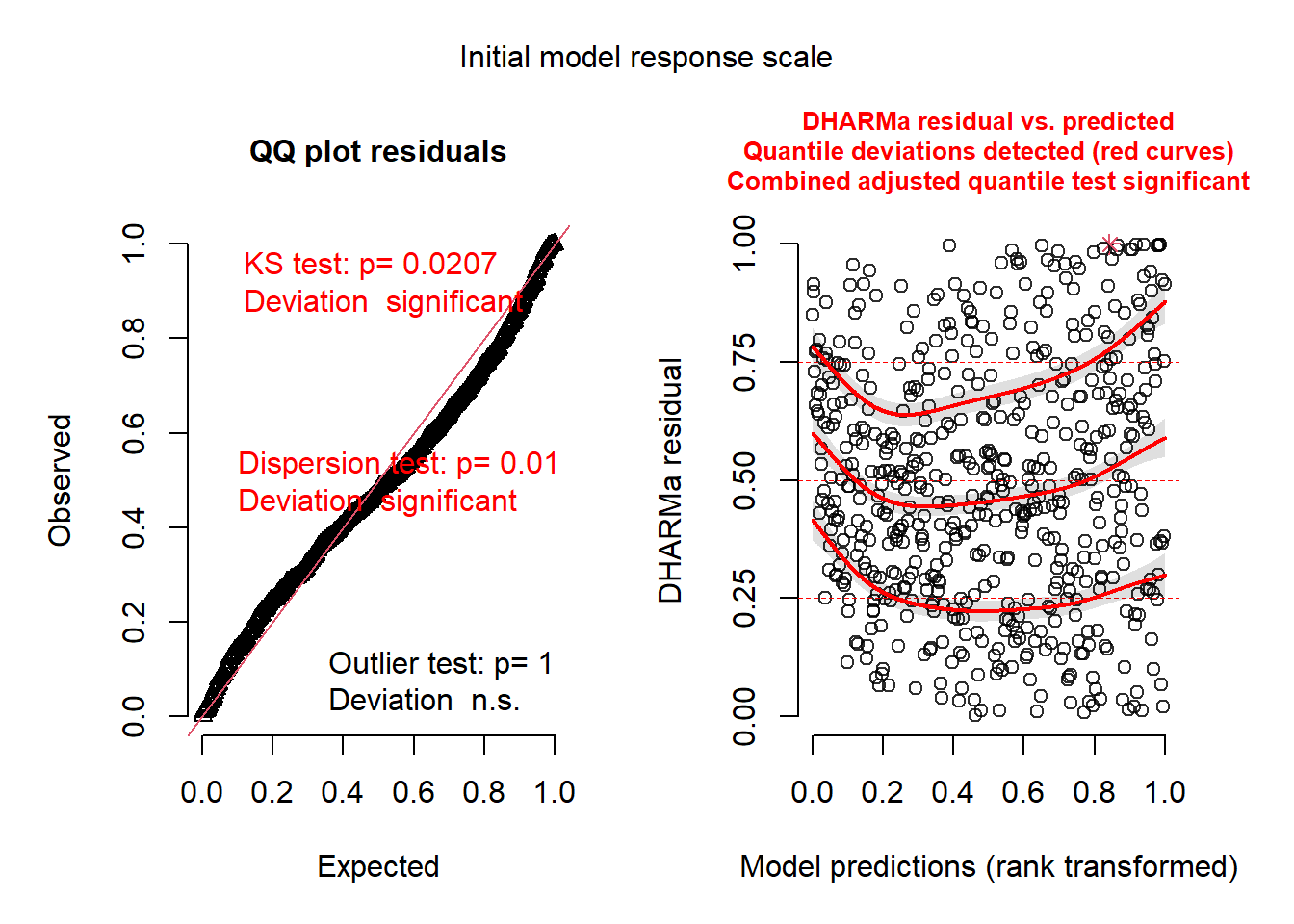
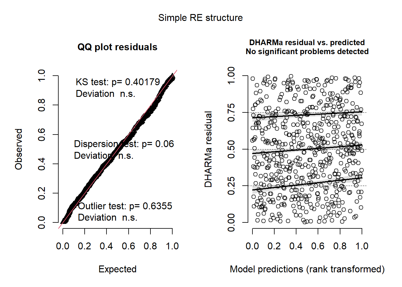
While the full model exhibited a significant dispersion result, potentially indicating some over specification in the random effects structure, the remaining diagnostic measures were satisfactory. Given that our primary focus was on predictive performance and we believe that the full RE structure is more representative of the data at hand we stuck with the full RE model.
ref_data<-copy(HIIR_dat)[,mu.vel_CV_SMF1 :=round(mean(mu.vel_CV_SMF1),2) ][,tm_CV_SMF1 :=round(mean(tm_CV_SMF1),2) ][,GH :=round(mean(GH),2) ][,.(Season,ID,GH,nsteps_CV_SMF1,mu.vel_CV_SMF1,tm_CV_SMF1)# create reference prediction based of average values ][,refPred_VT :=round(predict.gam(log_adj_VT_fin,.SD),2)# do some data cleaning for merging later ][,setnames(.SD,"mu.vel_CV_SMF1","mu_vel") ][,setnames(.SD,"tm_CV_SMF1","mu_time") ][,!c("GH","nsteps_CV_SMF1")]
Create a prediction grid based of observed values for that day
ind_pred = HIIR_dat[,.(Season,ID,GH,nsteps_CV_SMF1, pl.up_CV_SMF1,pl.fwd_CV_SMF1,pl.side_CV_SMF1, mu.vel_CV_SMF1,tm_CV_SMF1,logVT),# individual prediction: this would be extended fro AP and ML ][,indPred_VT :=round(predict.gam(log_adj_VT_fin),3)]
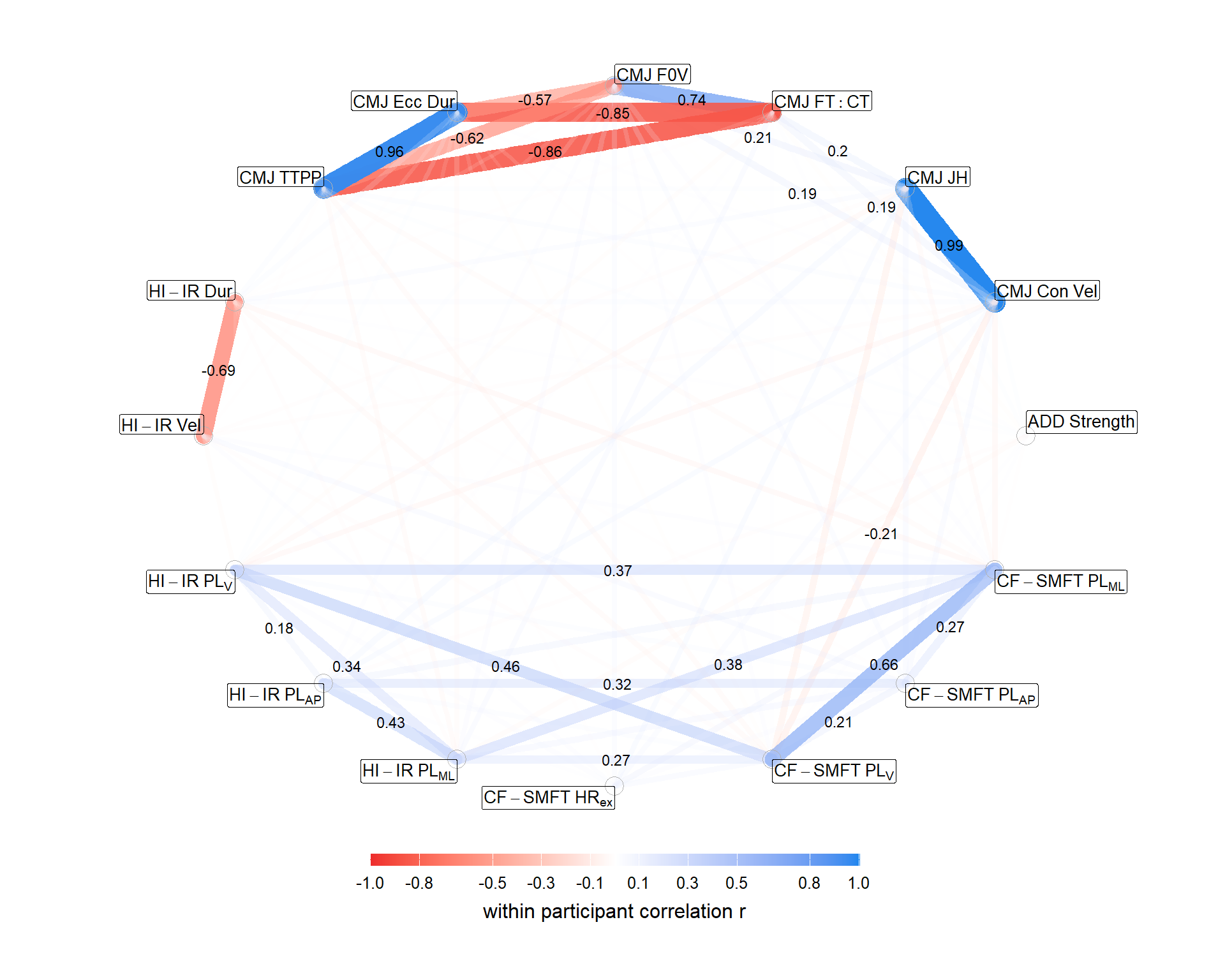
toi <-paste0("value_",c("ave_GB","ConPV_mx","JHIM.mx","FTCT.mx","FZVmx","EccDur.mn","TTPP.mn","tm_CV_SMF1","mu.vel_CV_SMF1","logAdj_pl.up","logAdj_pl.fwd","logAdj_pl.side","HRmu_perc","pl.up_CV_SMR1","pl.fwd_CV_SMR1","pl.side_CV_SMR1"))
Using the above data and to help contenxtulise results we ran a sensitivity analysis to given an indicator of the smallest correlation we could observed with 80% pwoer and at a alpha of 0.05.
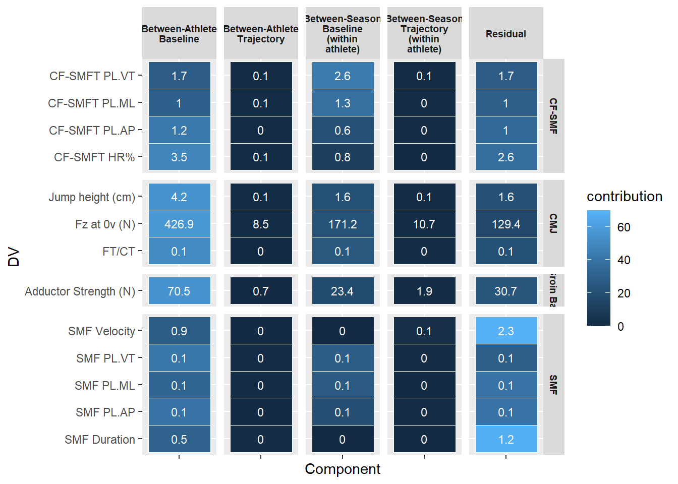
Between-Athlete Baseline: How much athletes differ from each other in their overall score. e.g. the between athlete SD across athletes for Jump height is 4.2cm
Between athlete Trajectory: How much athletes differ from each other in their rate of change over the season.
Between-Season baseline (within athlete): How much an individuals average performance varies between seasons.
Between-Season trajectory (within athlete): How much an individual rate of change varies between seasons.
Residual: Remaining variation within an athlete-season after accounting for all other patterns (within-subject variability)
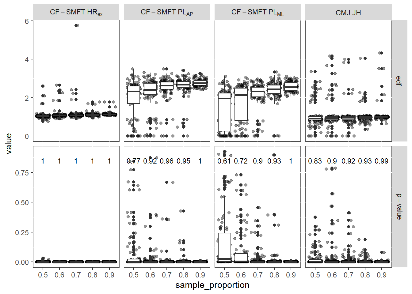
Running a sensitivity analysis for a GAM model is not as straight forward as for a linear model as the potential functional form is not known apriori. Instead, to provide insight into the stability of our model estimates, we performed a post-hoc sensitivity analysis. Specifically, we refitted the final model to multiple random subsamples of the data. To help contextualise the model’s stability, we have plotted the resulting distributions of the p-values and the Effective Degrees of Freedom (EDF) for our key predictors.
pacman::p_load(doSNOW,foreach,doParallel,progress)# Set up variablessubject_ids <-unique(CVTE_dat$ID)n_subjects <-length(subject_ids)vars <-c(2,10, 12,13)subsample_props <-c(0.5,0.6, 0.7, 0.8, 0.9)n_iterations <-100param_grid <-expand_grid(dependent_var_index = vars,prop = subsample_props,iteration =1:n_iterations)|>mutate(dependent_var_name = DVOI_scaled[dependent_var_index])## Helper function to run in parallel belowrun_single_model <-function(dv_name, proportion, iter_id) {# Set a seed for reproducibilityset.seed(iter_id *1000+ proportion *100) # Sample subjects subsample_ids <-sample(subject_ids, size =floor(n_subjects * proportion), replace =FALSE) sub_dat <- CVTE_dat[ID %in% subsample_ids, ]# Build and run the model formula_str <-paste0(dv_name, '~ s(Zscr_WI_TD_acu7,bs="ts")+ s(Zscr_WI_VHSR_25_acu7,bs="ts")+ s(Week,by=Season,bs="cs")+ s(ID, bs = "re")+ s(Week, ID, bs = "re")+ s(Week, Season, ID, bs = "re")+ s(Season, ID, bs = "re")') gam_subsample <-bam(as.formula(formula_str), data = sub_dat, discrete =TRUE, method ="fREML", select =TRUE)# Extract results and add metadata summary_df <-summary(gam_subsample)$s.table %>%as.data.frame() %>% tibble::rownames_to_column("var") %>%mutate(iteration = iter_id,sample_proportion = proportion,dependent_var = dv_name )return(summary_df)}## set up for parallel processingNCKF <-4# number of cores to keep free (update based on your computer)cl <-makeCluster(detectCores() - NCKF)registerDoSNOW(cl) # needs to be DoSnow for progress bar# create progress bar functionpb <- progress_bar$new(format ="Simulating [:bar] :percent | ETA: :eta",total =nrow(param_grid),width =80)progress_opts <-list(progress =function(n) pb$tick())# set up and runfinal_results_df <-foreach(i =1:nrow(param_grid),.combine ='rbind',.packages =c('mgcv', 'dplyr', 'tibble', 'data.table'),.export =c('run_single_model', 'subject_ids', 'n_subjects', 'CVTE_dat'),.options.snow = progress_opts) %dopar% {# Get parameters and run the model dv_name <- param_grid$dependent_var_name[i] proportion <- param_grid$prop[i] iter_id <- param_grid$iteration[i]run_single_model(dv_name, proportion, iter_id)}
Warning in dcast.data.table(.SD, dependent_var + dv + sample_proportion ~ :
'fun.aggregate' is NULL, but found duplicate row/column combinations, so
defaulting to length(). That is, the variables [dependent_var, dv,
sample_proportion, sig_flag] used in 'formula' do not uniquely identify rows in
the input 'data'. In such cases, 'fun.aggregate' is used to derive a single
representative value for each combination in the output data.table, for example
by summing or averaging (fun.aggregate=sum or fun.aggregate=mean,
respectively). Check the resulting table for values larger than 1 to see which
combinations were not unique. See ?dcast.data.table for more details.